Exploratory analysis using data summaries
Data sets can frequently be partitioned into meaningful groups based on the variables they contain. Making this grouping explicit allows the computation of numeric summaries within groups, which in turn facilitates quantitative comparisons.
This is the second module in the Visualization and EDA topic.
Overview
Learning Objectives
Conduct exploratory analyses using dplyr verbs
(group_by and summarize), along with numeric
data summaries.
Video Lecture
Example
We’ll continue in the same Git repo / R project that we used for
visualization, and use essentially the same weather_df
dataset – the only exception is the addition of month
variable, created using lubridate::floor_date().
library(p8105.datasets)
data("weather_df")

weather_df =
  weather_df |>
  mutate(
    month = lubridate::floor_date(date, unit = "month"))
Initial numeric explorations
Before beginning to summarize data, it can help to use initial visualizations to motivate some data checks or observations. Consider, for example, this histogram of precipitation values:
weather_df |>
  ggplot(aes(x = prcp)) +
  geom_histogram()
## `stat_bin()` using `bins = 30`. Pick better value with `binwidth`.
## Warning: Removed 15 rows containing non-finite outside the scale range
## (`stat_bin()`).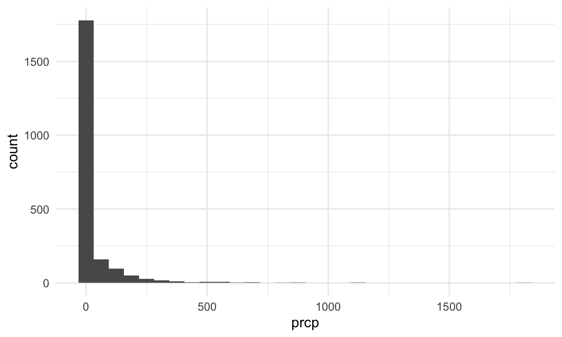
This is clearly a very skewed distribution; any formal analyses involving preciptation as a predictor or outcome might be influenced by this fact. It’s important to note that the vast majority of days have no precipitation. Meanwhile, examining the relatively few days have very high precipitation might be helpful.
weather_df |>
  filter(prcp >= 1000)
## # A tibble: 3 × 7
##   name           id          date        prcp  tmax  tmin month
##   <chr>          <chr>       <date>     <dbl> <dbl> <dbl> <date>
## 1 CentralPark_NY USW00094728 2021-08-21  1130  27.8  22.8 2021-08-01
## 2 CentralPark_NY USW00094728 2021-09-01  1811  25.6  17.2 2021-09-01
## 3 Molokai_HI     USW00022534 2022-12-18  1120  23.3  18.9 2022-12-01
The two high rainfall days in NYC correspond to tropical storm Henri and hurricane Ida, while the high precipitation day in Molokai took place during a notable cold front.
A close look at the scatterplot below (which focuses on a range of values to emphasize this point) suggests that Central Park and Molokai report temperature values differently from Waterhole …
weather_df |>
  filter(tmax >= 20, tmax <= 30) |>
  ggplot(aes(x = tmin, y = tmax, color = name, shape = name)) +
  geom_point(alpha = .75)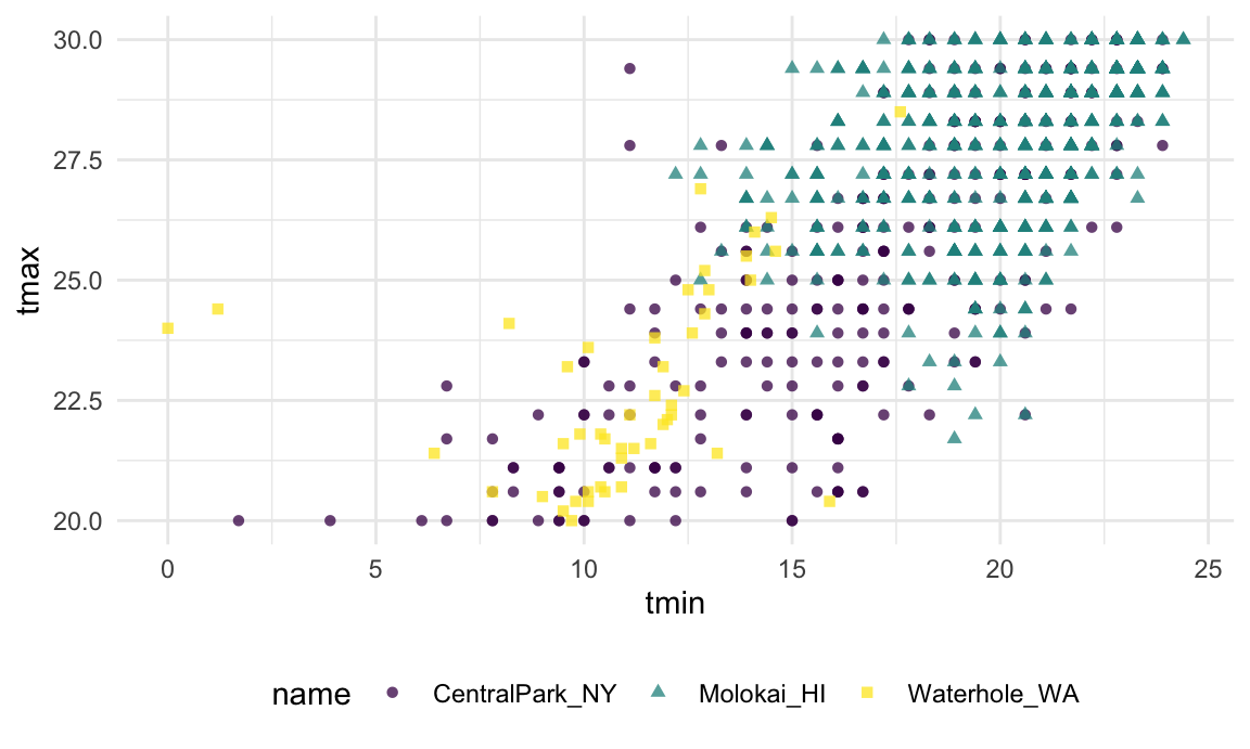
Depending on the nature of later analyses, understanding how these differ and implementing an approach to bring the reports into alignment might be necessary.
group_by
Datasets are often comprised of groups defined by one or more
(categorical) variable; group_by() makes these groupings
explicit so that they can be included in subsequent operations. For
example, we might group weather_df by name and
month:
weather_df |>
  group_by(name, month)
## # A tibble: 2,190 × 7
## # Groups:   name, month [72]
##   name           id          date        prcp  tmax  tmin month
##   <chr>          <chr>       <date>     <dbl> <dbl> <dbl> <date>
## 1 CentralPark_NY USW00094728 2021-01-01   157   4.4   0.6 2021-01-01
## 2 CentralPark_NY USW00094728 2021-01-02    13  10.6   2.2 2021-01-01
## 3 CentralPark_NY USW00094728 2021-01-03    56   3.3   1.1 2021-01-01
## 4 CentralPark_NY USW00094728 2021-01-04     5   6.1   1.7 2021-01-01
## 5 CentralPark_NY USW00094728 2021-01-05     0   5.6   2.2 2021-01-01
## 6 CentralPark_NY USW00094728 2021-01-06     0   5     1.1 2021-01-01
## # ℹ 2,184 more rows
Several important functions respect grouping structures. You will
frequently use summarize to create one-number summaries
within each group, or use mutate to define variables within
groups. The rest of this example shows these functions in action.
Because these (and other) functions will use grouping information if
it exists, it is sometimes necessary to remove groups using
ungroup().
Counting things
As an intro to summarize, let’s count the number of
observations in each month in the complete weather_df
dataset.
weather_df |>
  group_by(month) |>
  summarize(n_obs = n())
## # A tibble: 24 × 2
##   month      n_obs
##   <date>     <int>
## 1 2021-01-01    93
## 2 2021-02-01    84
## 3 2021-03-01    93
## 4 2021-04-01    90
## 5 2021-05-01    93
## 6 2021-06-01    90
## # ℹ 18 more rows
We can group by more than one variable, too.
weather_df |>
  group_by(name, month) |>
  summarize(n_obs = n())
## `summarise()` has grouped output by 'name'. You can override using the
## `.groups` argument.
## # A tibble: 72 × 3
## # Groups:   name [3]
##   name           month      n_obs
##   <chr>          <date>     <int>
## 1 CentralPark_NY 2021-01-01    31
## 2 CentralPark_NY 2021-02-01    28
## 3 CentralPark_NY 2021-03-01    31
## 4 CentralPark_NY 2021-04-01    30
## 5 CentralPark_NY 2021-05-01    31
## 6 CentralPark_NY 2021-06-01    30
## # ℹ 66 more rows
In both cases, the result is a dataframe that includes the grouping variable(s) and the desired summary.
To count things, you could use count() in place of
group_by() and summarize() if you remember
that this function exists. I’ll also make use of the name
argument in count, which defaults to "n".
weather_df |>
  count(month, name = "n_obs")
## # A tibble: 24 × 2
##   month      n_obs
##   <date>     <int>
## 1 2021-01-01    93
## 2 2021-02-01    84
## 3 2021-03-01    93
## 4 2021-04-01    90
## 5 2021-05-01    93
## 6 2021-06-01    90
## # ℹ 18 more rows
count() is a useful tidyverse alternative to Base R’s
table function. Both functions produce summaries of how
often values appear, but table’s output is of class
table and is hard to do any additional work with, while
count produces a dataframe you can use or manipulate
directly. For an example, run the code below and try to do something
useful with the result…
weather_df |>
  pull(month) |>
  table()
You can use summarize() to compute multiple summaries
within each group. As an example, we count the number of observations in
each month and the number of distinct values of date in
each month.
weather_df |>
  group_by(month) |>
  summarize(
    n_obs = n(),
    n_days = n_distinct(date))
## # A tibble: 24 × 3
##   month      n_obs n_days
##   <date>     <int>  <int>
## 1 2021-01-01    93     31
## 2 2021-02-01    84     28
## 3 2021-03-01    93     31
## 4 2021-04-01    90     30
## 5 2021-05-01    93     31
## 6 2021-06-01    90     30
## # ℹ 18 more rows
(2x2 tables)
You might find yourself, someday, wanting to tabulate the frequency
of a binary outcome across levels of a binary predictor. In a contrived
example, let’s say you want to look at the number of cold and not-cold
days in Central Park and Waterhole. We can do this with some extra data
manipulation steps and group_by +
summarize:
weather_df |>
  drop_na(tmax) |>
  mutate(
    cold = case_when(
      tmax <  5 ~ "cold",
      tmax >= 5 ~ "not_cold",
      TRUE      ~ ""
  )) |>
  filter(name != "Molokai_HI") |>
  group_by(name, cold) |>
  summarize(count = n())
## `summarise()` has grouped output by 'name'. You can override using the
## `.groups` argument.
## # A tibble: 4 × 3
## # Groups:   name [2]
##   name           cold     count
##   <chr>          <chr>    <int>
## 1 CentralPark_NY cold        96
## 2 CentralPark_NY not_cold   634
## 3 Waterhole_WA   cold       319
## 4 Waterhole_WA   not_cold   395
This is a “tidy” table, and it’s also a data frame. You could
re-organize into a more standard (non-tidy) 2x2 table using
pivot_wider, or you could use
janitor::tabyl:
weather_df |>
  drop_na(tmax) |>
  mutate(cold = case_when(
    tmax <  5 ~ "cold",
    tmax >= 5 ~ "not_cold",
    TRUE     ~ ""
  )) |>
  filter(name != "Molokai_HI") |>
  janitor::tabyl(name, cold)
##            name cold not_cold
##  CentralPark_NY   96      634
##    Waterhole_WA  319      395
This isn’t tidy, but it is still a data frame – and that’s noticeably
better than usual output from R’s built-in table function.
janitor has a lot of little functions like this that turn
out to be useful, so when you have some time you might read through all
the things you can do. I don’t really love that this is called
tabyl, but you can’t always get what you want in life.
(Since we’re on the subject, I think 2x2 tables are kind of silly. When are you ever going to actually analyze data in that format?? In grad school I thought I’d be computing odds ratios by hand everyday (\(OR = AD / BC\), right?!), but really I do that as often as I write in cursive – which is never. Just do a logistic regression adjusting for confounders – because there are always confounders. And is a 2x2 table really that much better than the “tidy” version? There are 4 numbers. )
General summaries
Standard statistical summaries are regularly computed in
summarize() using functions like mean(),
median(), var(), sd(),
mad(), IQR(), min(), and
max(). To use these, you indicate the variable to which
they apply and include any additional arguments as necessary.
weather_df |>
  group_by(month) |>
  summarize(
    mean_tmax = mean(tmax, na.rm = TRUE),
    mean_prec = mean(prcp, na.rm = TRUE),
    median_tmax = median(tmax),
    sd_tmax = sd(tmax))
## # A tibble: 24 × 5
##   month      mean_tmax mean_prec median_tmax sd_tmax
##   <date>         <dbl>     <dbl>       <dbl>   <dbl>
## 1 2021-01-01     10.9       39.5         5     12.2
## 2 2021-02-01      9.82      42.6         2.8   12.2
## 3 2021-03-01     13.7       55.5        NA     NA
## 4 2021-04-01     16.8       14.7        18.0    9.29
## 5 2021-05-01     19.6       17.3        22.2    9.40
## 6 2021-06-01     24.3       14.1        28.3    8.28
## # ℹ 18 more rows
You can group by more than one variable.
weather_df |>
  group_by(name, month) |>
  summarize(
    mean_tmax = mean(tmax),
    median_tmax = median(tmax))
## `summarise()` has grouped output by 'name'. You can override using the
## `.groups` argument.
## # A tibble: 72 × 4
## # Groups:   name [3]
##   name           month      mean_tmax median_tmax
##   <chr>          <date>         <dbl>       <dbl>
## 1 CentralPark_NY 2021-01-01      4.27         5
## 2 CentralPark_NY 2021-02-01      3.87         2.8
## 3 CentralPark_NY 2021-03-01     12.3         12.2
## 4 CentralPark_NY 2021-04-01     17.6         18.0
## 5 CentralPark_NY 2021-05-01     22.1         22.2
## 6 CentralPark_NY 2021-06-01     28.1         27.8
## # ℹ 66 more rows
If you want to summarize multiple columns using the same summary, the
across function is helpful.
weather_df |>
  group_by(name, month) |>
  summarize(across(tmin:prcp, mean))
## `summarise()` has grouped output by 'name'. You can override using the
## `.groups` argument.
## # A tibble: 72 × 5
## # Groups:   name [3]
##   name           month       tmin  tmax  prcp
##   <chr>          <date>     <dbl> <dbl> <dbl>
## 1 CentralPark_NY 2021-01-01 -1.15  4.27  18.9
## 2 CentralPark_NY 2021-02-01 -1.39  3.87  46.6
## 3 CentralPark_NY 2021-03-01  3.1  12.3   28.0
## 4 CentralPark_NY 2021-04-01  7.48 17.6   22.8
## 5 CentralPark_NY 2021-05-01 12.2  22.1   35.7
## 6 CentralPark_NY 2021-06-01 18.9  28.1   22.2
## # ℹ 66 more rows
The fact that summarize() produces a dataframe is
important (and consistent with other functions in the
tidyverse). You can incorporate grouping and summarizing
within broader analysis pipelines. For example, we can take create a
plot based on the monthly summary:
weather_df |>
  group_by(name, month) |>
  summarize(mean_tmax = mean(tmax, na.rm = TRUE)) |>
  ggplot(aes(x = month, y = mean_tmax, color = name)) +
    geom_point() + geom_line() +
    theme(legend.position = "bottom")
## `summarise()` has grouped output by 'name'. You can override using the
## `.groups` argument.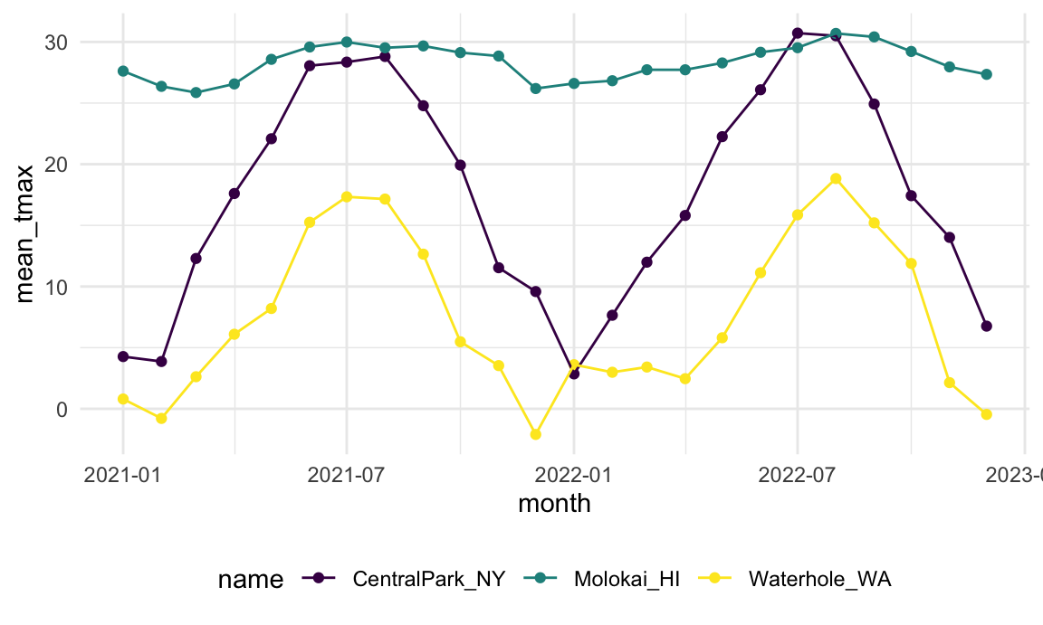
The results of group_by() and summarize()
are generally tidy, but presenting reader-friendly results for this kind
of exploratory analysis often benefits from some un-tidying. For
example, the table below shows month-by-month average max temperatures
in a more human-readable format.
weather_df |>
  group_by(name, month) |>
  summarize(mean_tmax = mean(tmax, na.rm = TRUE)) |>
  pivot_wider(
    names_from = name,
    values_from = mean_tmax) |>
  knitr::kable(digits = 1)
## `summarise()` has grouped output by 'name'. You can override using the
## `.groups` argument.| month | CentralPark_NY | Molokai_HI | Waterhole_WA |
|---|---|---|---|
| 2021-01-01 | 4.3 | 27.6 | 0.8 |
| 2021-02-01 | 3.9 | 26.4 | -0.8 |
| 2021-03-01 | 12.3 | 25.9 | 2.6 |
| 2021-04-01 | 17.6 | 26.6 | 6.1 |
| 2021-05-01 | 22.1 | 28.6 | 8.2 |
| 2021-06-01 | 28.1 | 29.6 | 15.3 |
| 2021-07-01 | 28.4 | 30.0 | 17.3 |
| 2021-08-01 | 28.8 | 29.5 | 17.2 |
| 2021-09-01 | 24.8 | 29.7 | 12.6 |
| 2021-10-01 | 19.9 | 29.1 | 5.5 |
| 2021-11-01 | 11.5 | 28.8 | 3.5 |
| 2021-12-01 | 9.6 | 26.2 | -2.1 |
| 2022-01-01 | 2.9 | 26.6 | 3.6 |
| 2022-02-01 | 7.7 | 26.8 | 3.0 |
| 2022-03-01 | 12.0 | 27.7 | 3.4 |
| 2022-04-01 | 15.8 | 27.7 | 2.5 |
| 2022-05-01 | 22.3 | 28.3 | 5.8 |
| 2022-06-01 | 26.1 | 29.2 | 11.1 |
| 2022-07-01 | 30.7 | 29.5 | 15.9 |
| 2022-08-01 | 30.5 | 30.7 | 18.8 |
| 2022-09-01 | 24.9 | 30.4 | 15.2 |
| 2022-10-01 | 17.4 | 29.2 | 11.9 |
| 2022-11-01 | 14.0 | 28.0 | 2.1 |
| 2022-12-01 | 6.8 | 27.3 | -0.5 |
Grouped mutate
Summarizing collapses groups into single data points. In contrast,
using mutate() in conjuntion with group_by()
will retain all original data points and add new variables computed
within groups.
Suppose you want to compare the daily max temperature to the annual average max temperature for each station separately, and to plot the result. You could do so using:
weather_df |>
  group_by(name) |>
  mutate(
    mean_tmax = mean(tmax, na.rm = TRUE),
    centered_tmax = tmax - mean_tmax) |>
  ggplot(aes(x = date, y = centered_tmax, color = name)) +
    geom_point()
## Warning: Removed 17 rows containing missing values or values outside the scale range
## (`geom_point()`).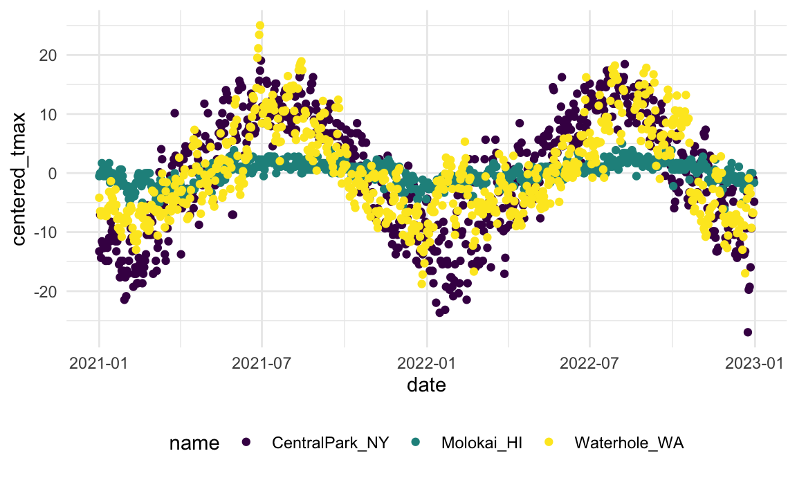
Window functions
The previous example used mean() to compute the mean
within each group, which was then subtracted from the observed max
tempurature. mean() takes n inputs and
produces a single output.
Window functions, in contrast, take n inputs and return
n outputs, and the outputs depend on all the inputs. There
are several categories of window functions; you’re most likely to need
ranking functions and offsets, which we illustrate below.
First, we can find the max temperature ranking within month.
weather_df |>
  group_by(name, month) |>
  mutate(temp_ranking = min_rank(tmax))
## # A tibble: 2,190 × 8
## # Groups:   name, month [72]
##   name           id         date        prcp  tmax  tmin month      temp_ranking
##   <chr>          <chr>      <date>     <dbl> <dbl> <dbl> <date>            <int>
## 1 CentralPark_NY USW000947… 2021-01-01   157   4.4   0.6 2021-01-01           14
## 2 CentralPark_NY USW000947… 2021-01-02    13  10.6   2.2 2021-01-01           31
## 3 CentralPark_NY USW000947… 2021-01-03    56   3.3   1.1 2021-01-01           13
## 4 CentralPark_NY USW000947… 2021-01-04     5   6.1   1.7 2021-01-01           20
## 5 CentralPark_NY USW000947… 2021-01-05     0   5.6   2.2 2021-01-01           19
## 6 CentralPark_NY USW000947… 2021-01-06     0   5     1.1 2021-01-01           16
## # ℹ 2,184 more rows
This sort of ranking is useful when filtering data based on rank. We could, for example, keep only the day with the lowest max temperature within each month:
weather_df |>
  group_by(name, month) |>
  filter(min_rank(tmax) < 2)
## # A tibble: 92 × 7
## # Groups:   name, month [72]
##   name           id          date        prcp  tmax  tmin month
##   <chr>          <chr>       <date>     <dbl> <dbl> <dbl> <date>
## 1 CentralPark_NY USW00094728 2021-01-29     0  -3.8  -9.9 2021-01-01
## 2 CentralPark_NY USW00094728 2021-02-08     0  -1.6  -8.2 2021-02-01
## 3 CentralPark_NY USW00094728 2021-03-02     0   0.6  -6   2021-03-01
## 4 CentralPark_NY USW00094728 2021-04-02     0   3.9  -2.1 2021-04-01
## 5 CentralPark_NY USW00094728 2021-05-29   117  10.6   8.3 2021-05-01
## 6 CentralPark_NY USW00094728 2021-05-30   226  10.6   8.3 2021-05-01
## # ℹ 86 more rows
We could also keep the three days with the highest max temperature:
weather_df |>
  group_by(name, month) |>
  filter(min_rank(desc(tmax)) < 4)
## # A tibble: 269 × 7
## # Groups:   name, month [72]
##   name           id          date        prcp  tmax  tmin month
##   <chr>          <chr>       <date>     <dbl> <dbl> <dbl> <date>
## 1 CentralPark_NY USW00094728 2021-01-02    13  10.6   2.2 2021-01-01
## 2 CentralPark_NY USW00094728 2021-01-14     0   9.4   3.9 2021-01-01
## 3 CentralPark_NY USW00094728 2021-01-16   198   8.3   2.8 2021-01-01
## 4 CentralPark_NY USW00094728 2021-02-16   208  10.6   1.1 2021-02-01
## 5 CentralPark_NY USW00094728 2021-02-24     0  12.2   3.9 2021-02-01
## 6 CentralPark_NY USW00094728 2021-02-25     0  10     4.4 2021-02-01
## # ℹ 263 more rows
In both of these, we’ve skipped a mutate() statement
that would create a ranking variable, and gone straight to filtering
based on the result.
Offsets, especially lags, are used to compare an observation to it’s previous value. This is useful, for example, to find the day-by-day change in max temperature within each station over the year:
weather_df |>
  group_by(name) |>
  mutate(temp_change = tmax - lag(tmax))
## # A tibble: 2,190 × 8
## # Groups:   name [3]
##   name           id          date        prcp  tmax  tmin month      temp_change
##   <chr>          <chr>       <date>     <dbl> <dbl> <dbl> <date>           <dbl>
## 1 CentralPark_NY USW00094728 2021-01-01   157   4.4   0.6 2021-01-01      NA
## 2 CentralPark_NY USW00094728 2021-01-02    13  10.6   2.2 2021-01-01       6.2
## 3 CentralPark_NY USW00094728 2021-01-03    56   3.3   1.1 2021-01-01      -7.3
## 4 CentralPark_NY USW00094728 2021-01-04     5   6.1   1.7 2021-01-01       2.8
## 5 CentralPark_NY USW00094728 2021-01-05     0   5.6   2.2 2021-01-01      -0.5
## 6 CentralPark_NY USW00094728 2021-01-06     0   5     1.1 2021-01-01      -0.600
## # ℹ 2,184 more rows
This kind of variable might be used to quantify the day-by-day variability in max temperature, or to identify the largest one-day increase:
weather_df |>
  group_by(name) |>
  mutate(temp_change = tmax - lag(tmax)) |>
  summarize(
    temp_change_sd = sd(temp_change, na.rm = TRUE),
    temp_change_max = max(temp_change, na.rm = TRUE))
## # A tibble: 3 × 3
##   name           temp_change_sd temp_change_max
##   <chr>                   <dbl>           <dbl>
## 1 CentralPark_NY           4.43            12.2
## 2 Molokai_HI               1.24             5.6
## 3 Waterhole_WA             3.04            11.1
Limitations
summarize() can only be used with functions that return
a single-number summary. This creates a ceiling, even if it is
very high. Later we’ll see how to aggregate data in a
more general way, and how to perform complex operations on the resulting
sub-datasets.
Revisiting examples
We’ve seen the PULSE and FAS datasets on several occasions, and we’ll briefly revisit them here.
Learning Assessment: In the PULSE data, the primary outcome is BDI score; it’s observed over follow-up visits, and we might ask if the typical BDI score values are roughly similar at each. Try to write a code chunk that imports, cleans, and summarizes the PULSE data to examine the mean and median at each visit. Export the results of this in a reader-friendly format.
Solution
The code chunk below imports and tidies the PUSLE data, produces the
desired information, and exports it using knitr::kable.
pulse_data =
  haven::read_sas("./data/public_pulse_data.sas7bdat") |>
  janitor::clean_names() |>
  pivot_longer(
    bdi_score_bl:bdi_score_12m,
    names_to = "visit",
    names_prefix = "bdi_score_",
    values_to = "bdi") |>
  select(id, visit, everything()) |>
  mutate(
    visit = replace(visit, visit == "bl", "00m"),
    visit = factor(visit, levels = str_c(c("00", "01", "06", "12"), "m"))) |>
  arrange(id, visit)

pulse_data |>
  group_by(visit) |>
  summarize(
    mean_bdi = mean(bdi, na.rm = TRUE),
    median_bdi = median(bdi, na.rm = TRUE)) |>
knitr::kable(digits = 3)Learning Assessment: In the FAS data, there are several outcomes of interest; for now, focus on post-natal day on which a pup is able to pivot. Two predictors of interest are the dose level and the day of treatment. Produce a reader-friendly table that quantifies the possible associations between dose, day of treatment, and the ability to pivot.
Solution
The code chunk below imports the litters and pups data, joins them,
produces the desired information, un-tidies the result, and exports a
table using knitr::kable.
pup_data =
  read_csv("./data/FAS_pups.csv", na = c("NA", "."), skip = 3) |>
  janitor::clean_names() |>
  mutate(sex = recode(sex, `1` = "male", `2` = "female"))

litter_data =
  read_csv("./data/FAS_litters.csv") |>
  janitor::clean_names() |>
  separate(group, into = c("dose", "day_of_tx"), sep = 3)

fas_data = left_join(pup_data, litter_data, by = "litter_number")

fas_data |>
  group_by(dose, day_of_tx) |>
  drop_na(dose) |>
  summarize(mean_pivot = mean(pd_pivot, na.rm = TRUE)) |>
  pivot_wider(
    names_from = dose,
    values_from = mean_pivot) |>
  knitr::kable(digits = 3)
These results may suggest that pups in the control group are able to pivot earlier than pups in the low-dose group, but it is unclear if there are differences between the control and moderate-dose groups or if day of treatment is an important predictor.
Note: In both of these examples, the data are structure such that repeated observations are made on the same study units. In the PULSE data, repeated observations are made on subjects over time; in the FAS data, pups are “repeated observations” within litters. The analyses here, and plots made previously, are exploratory – any more substantial claims would require appropriate statistical analysis for non-independent samples.
Other materials
- The preceding is based heavily on Jenny Bryan’s group_by material
- R for Data Science has sub-chapters on grouped summaries and exploratory data analysis
- A more in-depth overview of window functions is here
The code that I produced working examples in lecture is here.