Iteration and List Columns
We’ve noted that functions are helpful when you repeat code more than twice; we’ve also noted that a lot of statistical methods involve doing the same thing a large number of times. Putting those together motivates a careful approach to iteratation.
Meanwhile, R’s data structures, especially data frames, are
surprisingly flexible. This is useful when the “observations” you want
to store become more complex than single values; for example, each row
many contain a few scalar observations as well a complete data set. In
these cases, list columns are an appropriate column type, and
map functions provide a way to interact with those
columns.
This is the second module in the Iteration topic.
Overview
Learning Objectives
There are stops along the way, but our goal is to use map functions and iterate over listcolumns in data frames.
Video Lecture
Example
I’ll write code for today’s content in a new R Markdown document
called iteration_and_listcols.Rmd in the
iteration repo / directory I started last time. The code
chunk below loads the tidyverse and sets a seed for
reproducibility.
library(tidyverse)
library(rvest)
##
## Attaching package: 'rvest'## The following object is masked from 'package:readr':
##
## guess_encodingset.seed(1)Things are gonna get a little weird…
Lists
We need a brief digression about lists before we do anything.
In R, vectors are limited to a single data class – all elements are characters, or all numeric, or all logical. Trying to join the following vectors will result in coersion, as would creating vectors of mixed types.
vec_numeric = 5:8
vec_char = c("My", "name", "is", "Jeff")
vec_logical = c(TRUE, TRUE, TRUE, FALSE)
Lists provide a way to store anything you want. This flexibility is great, but is offset by a certain … clunkiness. Lists contain indexed elements, and the indexed elements themselves be scalars, vectors, or other things entirely.
l = list(
  vec_numeric = 5:8,
  mat         = matrix(1:8, 2, 4),
  vec_logical = c(TRUE, FALSE),
  summary     = summary(rnorm(1000)))
l
## $vec_numeric
## [1] 5 6 7 8
##
## $mat
## [,1] [,2] [,3] [,4]
## [1,] 1 3 5 7
## [2,] 2 4 6 8
##
## $vec_logical
## [1] TRUE FALSE
##
## $summary
## Min. 1st Qu. Median Mean 3rd Qu. Max.
## -3.00805 -0.69737 -0.03532 -0.01165 0.68843 3.81028Lists can be accessed using names or indices, and the things in lists can be accessed in the way you would usually access an object of that type.
l$vec_numeric## [1] 5 6 7 8l[[1]]## [1] 5 6 7 8l[[1]][1:3]## [1] 5 6 7Lists seem bizarre but are really useful. Right now, we’ll use them to hold general inputs and outputs of iterative processes. Even more importantly, we’ll see that data frames are actually a very specific kind of list – one comprised of vectors of the same length – which is why they can store variables of different types.
for loops
For this example, I’m going to start with the list defined below.
list_norms =
  list(
    a = rnorm(20, 3, 1),
    b = rnorm(20, 0, 5),
    c = rnorm(20, 10, .2),
    d = rnorm(20, -3, 1)
  )

is.list(list_norms)
## [1] TRUEI’d like to apply my simple mean_and_sd function from writing functions to each element of
this list For completeness, that function is below.
mean_and_sd = function(x) {

  if (!is.numeric(x)) {
    stop("Argument x should be numeric")
  } else if (length(x) == 1) {
    stop("Cannot be computed for length 1 vectors")
  }

  mean_x = mean(x)
  sd_x = sd(x)

  tibble(
    mean = mean_x,
    sd = sd_x
  )
}
We can apply the mean_and_sd function to each element of
list_norms using the lines below.
mean_and_sd(list_norms[[1]])## # A tibble: 1 × 2
## mean sd
## <dbl> <dbl>
## 1 2.70 1.12mean_and_sd(list_norms[[2]])## # A tibble: 1 × 2
## mean sd
## <dbl> <dbl>
## 1 0.416 4.08mean_and_sd(list_norms[[3]])## # A tibble: 1 × 2
## mean sd
## <dbl> <dbl>
## 1 10.1 0.191mean_and_sd(list_norms[[4]])## # A tibble: 1 × 2
## mean sd
## <dbl> <dbl>
## 1 -3.43 1.18But now we’ve broken our “don’t repeat code more than twice” rule! Specifically, we’ve applied the same function / operation to the elements of a list sequentially. This is exactly the kind of code repetition for loops address
Below, I define an output list with the same number of entries as my
target dataframe; a sequence to iterate over; and a for loop body that
applies the mean_and_sd function for each sequence element
and saves the result.
output = vector("list", length = 4)
for (i in 1:4) {
output[[i]] = mean_and_sd(list_norms[[i]])
}This is already much cleaner than using four almost-identical lines of code, and will make life easier the larger our sequence gets.
In this example, I bypassed a common first step in writing loops because I already had the function I wanted to repeat. Frequently, however, I’ll start with repeated code segements, then abstract the underlying process into a function, and then wrap things up in a for loop.
map
A criticism of for loops is that there’s a lot of
overhead – you have to define your output vector / list, there’s the
for loop bookkeeping to do, etc – that distracts from the
purpose of the code. In this case, we want to apply
mean_and_sd to each element of list_norms, but
we have to scan inside the for loop to figure that out.
The map functions in purrr try to make the
purpose of your code clear. Compare the loop above to the line
below.
output = map(list_norms, mean_and_sd)The first argument to map is the list (or vector, or
data frame) we want to iterate over, and the second argument is the
function we want to apply to each element. The line above will produce
the same output as the previous loop, but is clearer and easier to
understand (once you’re used to map …).
This code (using map) is why we pointed out in writing functions that functions can
be passed as arguments to other functions. The second argument in
map(list_norms, mean_and_sd) is a function we just wrote.
To see how powerful this can be, suppose we wanted to apply a different
function, say median, to each column of
list_norms. The chunk below includes both the loop and the
map approach.
output = vector("list", length = 4)
for (i in 1:4) {
output[[i]] = median(list_norms[[i]])
}
output = map(list_norms, median)Again, both options produce the same output, but the
map places the focus squarely on the function you want to
apply by removing much of the bookkeeping.
map variants
There are some useful variants to the basic map function
if you know what kind of output you’re going to produce. Below we use
map_dbl because median outputs a single
numeric value each time; the result is a vector instead of a list. Using
the .id argument keeps the names of the elements in the
input list.
output = map_dbl(list_norms, median, .id = "input")If we tried to use map_int or map_lgl, we’d
get an error because the output of median isn’t a integer
or a logical. This is a good way to help catch mistakes when they
arise.
Similarly, since we know mean_and_sd produces a data
frame, we can use the output-specific map_dfr; this will
produce a single data frame.
output = map_dfr(list_norms, mean_and_sd, .id = "input")The map_df variants can be helpful when your map
statement is part of a longer chain of piped commands.
Lastly, the variant map2 (and map2_dbl,
etc) is helpful when your function has two arguments. In these cases, I
find it best to be specific about arguments using something like the
following (more on anonymous functions shortly):
output = map2(input_1, input_2, \(x,y) func(arg_1 = x, arg_2 = y))List columns and operations
listcol_df =
tibble(
name = c("a", "b", "c", "d"),
samp = list_norms
)The name column is a character column – if you pull this
column from the listcol_df data frame, the result is a
character vector. Similarly, the samp column is a list
column – on it’s own, it’s a list.
listcol_df |> pull(name)## [1] "a" "b" "c" "d"listcol_df |> pull(samp)## $a
## [1] 4.134965 4.111932 2.129222 3.210732 3.069396 1.337351 3.810840 1.087654
## [9] 1.753247 3.998154 2.459127 2.783624 1.378063 1.549036 3.350910 2.825453
## [17] 2.408572 1.665973 1.902701 5.036104
##
## $b
## [1] -1.63244797 3.87002606 3.92503200 3.81623040 1.47404380 -6.26177962
## [7] -5.04751876 3.75695597 -6.54176756 2.63770049 -2.66769787 -1.99188007
## [13] -3.94784725 -1.15070568 4.38592421 2.26866589 -1.16232074 4.35002762
## [19] 8.28001867 -0.03184464
##
## $c
## [1] 10.094098 10.055644 9.804419 9.814683 10.383954 10.176256 10.148416
## [8] 10.029515 10.097078 10.030371 10.008400 10.044684 9.797907 10.480244
## [15] 10.160392 9.949758 10.242578 9.874548 10.342232 9.921125
##
## $d
## [1] -5.321491 -1.635881 -1.867771 -3.774316 -4.410375 -4.834528 -3.269014
## [8] -4.833929 -3.814468 -2.836428 -2.144481 -3.819963 -3.123603 -2.745052
## [15] -1.281074 -3.958544 -4.604310 -4.845609 -2.444263 -3.060119The list column really is a list, and will behave as such elsewhere in R. So, for example, you can examine the first list entry using usual list index procedures.
pull(listcol_df, samp)[[1]]## [1] 4.134965 4.111932 2.129222 3.210732 3.069396 1.337351 3.810840 1.087654
## [9] 1.753247 3.998154 2.459127 2.783624 1.378063 1.549036 3.350910 2.825453
## [17] 2.408572 1.665973 1.902701 5.036104You will need to be able to manipulate list columns, but usual
operations for columns that might appear in mutate (like
mean or recode) often don’t apply to the
entries in a list column. Instead, recognizing list columns as
list columns motivates an approach for working
with them.
Let’s apply mean_and_sd to the first element of our list
column.
mean_and_sd(pull(listcol_df, samp)[[1]])## # A tibble: 1 × 2
## mean sd
## <dbl> <dbl>
## 1 2.70 1.12Great! Keeping in mind that pull(listcol_df, samp) is a
list, we can apply mean_and_sd
function to each element using map.
map(pull(listcol_df, samp), mean_and_sd)## $a
## # A tibble: 1 × 2
##    mean    sd
##   <dbl> <dbl>
## 1  2.70  1.12
##
## $b
## # A tibble: 1 × 2
##    mean    sd
##   <dbl> <dbl>
## 1 0.416  4.08
##
## $c
## # A tibble: 1 × 2
##    mean    sd
##   <dbl> <dbl>
## 1  10.1 0.191
##
## $d
## # A tibble: 1 × 2
##    mean    sd
##   <dbl> <dbl>
## 1 -3.43 1.18The map function returns a list; we could store
the results as a new list column … !!!
We’ve been using mutate to define a new variable in a
data frame, especially one that is a function of an existing variable.
That’s exactly what we will keep doing.
listcol_df =
  listcol_df |>
  mutate(summary = map(samp, mean_and_sd))

listcol_df
## # A tibble: 4 × 3
## name samp summary
## <chr> <named list> <named list>
## 1 a <dbl [20]> <tibble [1 × 2]>
## 2 b <dbl [20]> <tibble [1 × 2]>
## 3 c <dbl [20]> <tibble [1 × 2]>
## 4 d <dbl [20]> <tibble [1 × 2]>Revisiting NSDUH
In reading data from the
web and elsewhere, we wrote code that allowed us to import data
tables from a recent NSDUH survey; in writing functions we wrapped that code
into a function called nsduh_table which, for a given
table_number, produces a data frame containing state, age
group, year, and percents. A similar function, which omits the argument
table_name, is shown below.
nsduh_table <- function(html, table_num) {

  table =
    html |>
    html_table() |>
    nth(table_num) |>
    slice(-1) |>
    select(-contains("P Value")) |>
    pivot_longer(
      -State,
      names_to = "age_year",
      values_to = "percent") |>
    separate(age_year, into = c("age", "year"), sep = "\\(") |>
    mutate(
      year = str_replace(year, "\\)", ""),
      percent = str_replace(percent, "[a-c]$", ""),
      percent = as.numeric(percent)) |>
    filter(!(State %in% c("Total U.S.", "Northeast", "Midwest", "South", "West")))

  table
}
We can use this function to import three tables using the next code
chunk, which downloads and extracts the page HTML and then iterates over
table numbers. The results are combined using bind_rows().
Note that, because this version of our function doesn’t include
table_name, that information is lost for now.
nsduh_url = "http://samhda.s3-us-gov-west-1.amazonaws.com/s3fs-public/field-uploads/2k15StateFiles/NSDUHsaeShortTermCHG2015.htm"

nsduh_html = read_html(nsduh_url)

output = vector("list", 3)

for (i in c(1, 4, 5)) {
  output[[i]] = nsduh_table(nsduh_html, i)
}

nsduh_results = bind_rows(output)
We can also import these data using map(). Here I’m
supplying the html argument after the name of the function
that I’m iterating over.
nsduh_results =
  map(c(1, 4, 5), nsduh_table, html = nsduh_html) |>
  bind_rows()
As with previous examples, using a for loop is pretty okay but the
map call is clearer.
We can also do this using data frames and list columns. Here, we’re
mapping over number, applying the nsduh_table
function, and then indicating that the html argument in
that function should always be set to nsduh_html. This is
necessary because our function has two arguments, and map
won’t know where to put number without some additional
information.
nsduh_results=
  tibble(
    name = c("marj", "cocaine", "heroine"),
    number = c(1, 4, 5)) |>
  mutate(table = map(number, nsduh_table, html = nsduh_html)) |>
  unnest(cols = "table")
An alternative way to accomplish this is to use map’s
syntax for “anonymous” (i.e. not named and saved) functions. This is
helpful for really short operations – here, we’re indicating that the
only argument to care about is num and then passing that
into nsduh_html.
nsduh_results=
  tibble(
    name = c("marj", "cocaine", "heroine"),
    number = c(1, 4, 5)) |>
  mutate(table = map(number, \(num) nsduh_table(html = nsduh_html, num))) |>
  unnest(cols = "table")
Operations on nested data
Shifting gears a bit, let’s revisit the weather data from visualization and elsewhere; these data
consist of one year of observations from three monitoring stations. The
code below pulls these data into R using the p8105.datasets
package.
library(p8105.datasets)
data("weather_df")
The station name and id are constant across the year’s temperature and precipitation data. For that reason, we can reorganize these data into a new data frame with a single row for each station. Weather data will be separated into three station-specific data frames, each of which is the data “observation” for the respective station.
weather_nest =
  nest(weather_df, data = date:tmin)

weather_nest
## # A tibble: 3 × 3
## name id data
## <chr> <chr> <list>
## 1 CentralPark_NY USW00094728 <tibble [730 × 4]>
## 2 Molokai_HI USW00022534 <tibble [730 × 4]>
## 3 Waterhole_WA USS0023B17S <tibble [730 × 4]>This is a different way of producing a list column. The result is a
lot like listcol_df, in that the columns in
weather_nest are a vector and a list.
weather_nest |> pull(name)## [1] "CentralPark_NY" "Molokai_HI" "Waterhole_WA"weather_nest |> pull(data)## [[1]]
## # A tibble: 730 × 4
## date prcp tmax tmin
## <date> <dbl> <dbl> <dbl>
## 1 2021-01-01 157 4.4 0.6
## 2 2021-01-02 13 10.6 2.2
## 3 2021-01-03 56 3.3 1.1
## 4 2021-01-04 5 6.1 1.7
## 5 2021-01-05 0 5.6 2.2
## 6 2021-01-06 0 5 1.1
## 7 2021-01-07 0 5 -1
## 8 2021-01-08 0 2.8 -2.7
## 9 2021-01-09 0 2.8 -4.3
## 10 2021-01-10 0 5 -1.6
## # ℹ 720 more rows
##
## [[2]]
## # A tibble: 730 × 4
## date prcp tmax tmin
## <date> <dbl> <dbl> <dbl>
## 1 2021-01-01 0 27.8 22.2
## 2 2021-01-02 0 28.3 23.9
## 3 2021-01-03 0 28.3 23.3
## 4 2021-01-04 0 30 18.9
## 5 2021-01-05 0 28.9 21.7
## 6 2021-01-06 0 27.8 20
## 7 2021-01-07 0 29.4 21.7
## 8 2021-01-08 0 28.3 18.3
## 9 2021-01-09 0 27.8 18.9
## 10 2021-01-10 0 28.3 18.9
## # ℹ 720 more rows
##
## [[3]]
## # A tibble: 730 × 4
## date prcp tmax tmin
## <date> <dbl> <dbl> <dbl>
## 1 2021-01-01 254 3.2 0
## 2 2021-01-02 152 0.9 -3.2
## 3 2021-01-03 0 0.2 -4.2
## 4 2021-01-04 559 0.9 -3.2
## 5 2021-01-05 25 0.5 -3.3
## 6 2021-01-06 51 0.8 -4.8
## 7 2021-01-07 0 0.2 -5.8
## 8 2021-01-08 25 0.5 -8.3
## 9 2021-01-09 0 0.1 -7.7
## 10 2021-01-10 203 0.9 -0.1
## # ℹ 720 more rowsOf course, if you can nest data you should be able to
unnest it as well, and you can (with the caveat that you’re
unnesting a list column that contains a data frame).
unnest(weather_nest, cols = data)## # A tibble: 2,190 × 6
## name id date prcp tmax tmin
## <chr> <chr> <date> <dbl> <dbl> <dbl>
## 1 CentralPark_NY USW00094728 2021-01-01 157 4.4 0.6
## 2 CentralPark_NY USW00094728 2021-01-02 13 10.6 2.2
## 3 CentralPark_NY USW00094728 2021-01-03 56 3.3 1.1
## 4 CentralPark_NY USW00094728 2021-01-04 5 6.1 1.7
## 5 CentralPark_NY USW00094728 2021-01-05 0 5.6 2.2
## 6 CentralPark_NY USW00094728 2021-01-06 0 5 1.1
## 7 CentralPark_NY USW00094728 2021-01-07 0 5 -1
## 8 CentralPark_NY USW00094728 2021-01-08 0 2.8 -2.7
## 9 CentralPark_NY USW00094728 2021-01-09 0 2.8 -4.3
## 10 CentralPark_NY USW00094728 2021-01-10 0 5 -1.6
## # ℹ 2,180 more rowsNesting columns can help with data organization and comprehension by masking complexity you’re less concerned about right now and clarifying the things you are concerned about. In the weather data, it can be helpful to think of stations as the basic unit of observation, and daily weather recordings as a more granular level of observation. Nesting can also simplify the use of analytic approaches across levels of a higher variable.
Suppose we want to fit the simple linear regression relating
tmax to tmin for each station-specific data
frame. First I’ll write a quick function that takes a data frame as the
sole argument to fit this model.
weather_lm = function(df) {
  lm(tmax ~ tmin, data = df)
}
Let’s make sure this works on a single data frame.
weather_lm(pull(weather_nest, data)[[1]])##
## Call:
## lm(formula = tmax ~ tmin, data = df)
##
## Coefficients:
## (Intercept) tmin
## 7.514 1.034Since pull(weather_nest, data) is a
list, we can apply our weather_lm
function to each data frame using map.
map(pull(weather_nest, data), weather_lm)## [[1]]
##
## Call:
## lm(formula = tmax ~ tmin, data = df)
##
## Coefficients:
## (Intercept)         tmin
##       7.514        1.034
##
##
## [[2]]
##
## Call:
## lm(formula = tmax ~ tmin, data = df)
##
## Coefficients:
## (Intercept) tmin
## 21.7547 0.3222
##
##
## [[3]]
##
## Call:
## lm(formula = tmax ~ tmin, data = df)
##
## Coefficients:
## (Intercept) tmin
## 7.532 1.137Again, you can avoid the creation of a dedicated function using
map’s syntax for “anonymous” (i.e. not named and saved)
functions. This is helpful for really short operations – here, rather
than writing a separate (named) function that takes the argument
df and returns a regression of tmax on
tmin, I can use \(df) to indicate that same
function. If you have a one-line function, this is a good option;
otherwise creating a named function is probably better.
map(pull(weather_nest, data), \(df) lm(tmax ~ tmin, data = df))## [[1]]
##
## Call:
## lm(formula = tmax ~ tmin, data = df)
##
## Coefficients:
## (Intercept) tmin
## 7.514 1.034
##
##
## [[2]]
##
## Call:
## lm(formula = tmax ~ tmin, data = df)
##
## Coefficients:
## (Intercept) tmin
## 21.7547 0.3222
##
##
## [[3]]
##
## Call:
## lm(formula = tmax ~ tmin, data = df)
##
## Coefficients:
## (Intercept) tmin
## 7.532 1.137Let’s use mutate to fit this model, and to store the
result in the same dataframe.
weather_nest =
  weather_nest |>
  mutate(models = map(data, weather_lm))

weather_nest
## # A tibble: 3 × 4
## name id data models
## <chr> <chr> <list> <list>
## 1 CentralPark_NY USW00094728 <tibble [730 × 4]> <lm>
## 2 Molokai_HI USW00022534 <tibble [730 × 4]> <lm>
## 3 Waterhole_WA USS0023B17S <tibble [730 × 4]> <lm>This is great! We now have a data frame that has rows for each station; columns contain weather datasets and fitted models. This makes it very easy to keep track of models across stations, and to perform additional analyses.
This is, for sure, a fairly complex bit of code, but in just a few
lines we’re able to fit separate linear models to each of our stations.
And, once you get used to list columns, map, and the rest
of it, these lines of code are pretty clear and can be extended to
larger datasets with more complex structures.
Using iteration for data import
This zip file contains data from a longitudinal study that included a control arm and an experimental arm. Data for each participant is included in a separate file, and file names include the subject ID and arm.
The code chunk below imports the data in individual spreadsheets
contained in ./data/zip_data/. To do this, I create a
dataframe that includes the list of all files in that directory and the
complete path to each file. As a next step, I map over
paths and import data using the read_csv function. Finally,
I unnest the result of map.
full_df =
  tibble(
    files = list.files("data/exp_data/"),
    path = str_c("data/exp_data/", files)
  ) %>%
  mutate(data = map(path, read_csv)) %>%
  unnest()
## Rows: 1 Columns: 8
## ── Column specification ────────────────────────────────────────────────────────
## Delimiter: ","
## dbl (8): week_1, week_2, week_3, week_4, week_5, week_6, week_7, week_8
##
## ℹ Use `spec()` to retrieve the full column specification for this data.
## ℹ Specify the column types or set `show_col_types = FALSE` to quiet this message.
## Rows: 1 Columns: 8
## ── Column specification ────────────────────────────────────────────────────────
## Delimiter: ","
## dbl (8): week_1, week_2, week_3, week_4, week_5, week_6, week_7, week_8
##
## ℹ Use `spec()` to retrieve the full column specification for this data.
## ℹ Specify the column types or set `show_col_types = FALSE` to quiet this message.The result of the previous code chunk isn’t tidy – data are wide rather than long, and some important variables are included as parts of others. The code chunk below tides the data using string manipulations on the file, converting from wide to long, and selecting relevant variables.
tidy_df =
  full_df %>%
  mutate(
    files = str_replace(files, ".csv", ""),
    group = str_sub(files, 1, 3)) %>%
  pivot_longer(
    week_1:week_8,
    names_to = "week",
    values_to = "outcome",
    names_prefix = "week_") %>%
  mutate(week = as.numeric(week)) %>%
  select(group, subj = files, week, outcome)
Finally, the code chunk below creates a plot showing individual data, faceted by group.
tidy_df %>%
  ggplot(aes(x = week, y = outcome, group = subj, color = group)) +
  geom_point() +
  geom_path() +
  facet_grid(~group)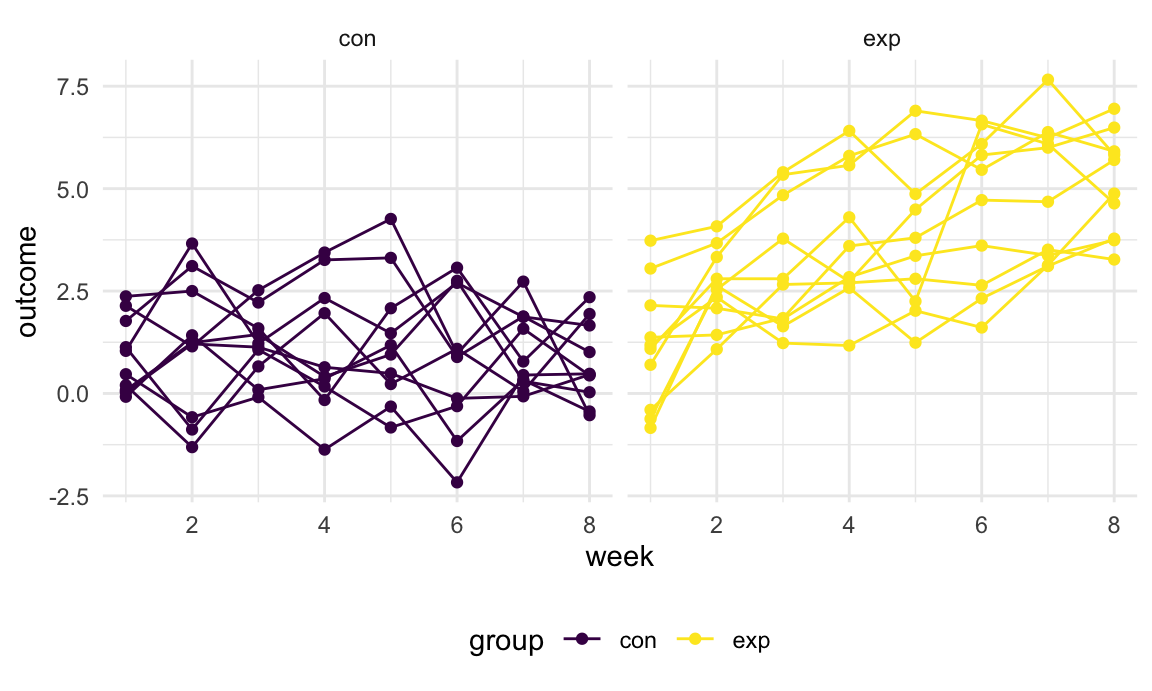
This plot suggests high within-subject correlation – subjects who start above average end up above average, and those that start below average end up below average. Subjects in the control group generally don’t change over time, but those in the experiment group increase their outcome in a roughly linear way.
Other materials
Iteration can be tricky – the readings below will help as you work through this!
- The chapter on iteration in R for Data
Science has a useful treatment of iteration using loops and
map - Jenny Bryan’s
purrrtutorial has a lot of useful information and examples - R Programming for Data Science has information on loops
and loop
functions; given Roger Peng’s tendency towards base R he focuses on
lapplyand others instead ofmap - This question
and response on stack overflow explains why one might prefer
maptolapply
List columns take some getting used to; there are some materials to help with that.
- R for Data Science has a chapter on fitting many models
- Jenny Bryan’s purrr tutorial has useful list-column examples
- The R
file used to create the
starwarsdataset (in thetidyverse) using the Star Wars API processes list output (from the API) using severalmapvariants
The code that I produced working examples in lecture is here.