Simulation

We’ve noted that functions are helpful when you repeat code more than twice; we’ve also noted that a lot of statistical methods involve doing the same thing a large number of times. Simulation is a common statistical approach that takes advantage of the ability to iterate many times using computers.

This is the third module in the Iteration topic.

Overview

Learning Objectives

Use iteration methods to simulate data, and explore statistical properties of common estimation methods under repeated sampling using simulations.

Slide Deck

Simulation from Jeff Goldsmith.

---

Video Lecture

---

Example

I’ll write code for today’s content in a new R Markdown document called simulation.Rmd in the iteration directory / repo. The code chunk below loads the usual packages and sets a seed for reproducibility.

library(tidyverse)

set.seed(1)

Simulation: Mean and SD for one \(n\)

In writing functions we wrote a short function to simulate data from a normal distribution, and return estimates of the mean and standard deviation. Specifically, we generate data from \[ x_i \sim N[\mu, \sigma] \]

for subjects \(1 \leq i \leq n\) and return estimates

\(\hat{\mu}, \hat{\sigma}\). That function is below.

sim_mean_sd = function(n, mu = 2, sigma = 3) {
  
  sim_data = tibble(
    x = rnorm(n, mean = mu, sd = sigma),
  )
  
  sim_data |> 
    summarize(
      mu_hat = mean(x),
      sigma_hat = sd(x)
    )
}

Important statistical properties of estimates \(\hat{\mu}\) are established under the conceptual framework of repeated sampling. If you could draw from a population over and over, your estimates will have a known distribution:

\[ \hat{\mu} \sim \left[\mu,\frac{\sigma}{\sqrt{n}} \right]\]

Because our simulation design generates observations from a Normal distribution we also know that the estimates follow a Normal distribution, although that’s not guaranteed in general. You can do some work to understand the distribution of \(\hat{\sigma}\), but it’s … messier.

In the real world, drawing samples is time consuming and costly, so “repeated sampling” remains conceptual. On a computer, though, drawing samples is pretty easy. That makes simulation an appealing way to examine the statistical properties of your estimators.

Let’s run sim_mean_sd() 100 times to see the effect of randomness in \(x_i\) on estimates \(\hat{\mu}, \hat{\sigma}\).

output = vector("list", 100)

for (i in 1:100) {
  output[[i]] = sim_mean_sd(30)
}

sim_results = bind_rows(output)

Taking a look at the for loop we used to create these results, you might notice that there’s no input list – the sequence is used to keep track of the output but doesn’t affect the computation performed inside the for loop. We can still use map to carry this out, of course – we’ll just be mapping over something that doesn’t change.

In the code below, I create a data frame with rows for 100 iterations; the sample size column is fixed at 30 in every row. Then, using ideas from iteration and list columns, I’ll map my sim_mean_sd function over the sample_size column to replicate the simulation in the previous loop.

sim_results_df = 
  expand_grid(
    sample_size = 30,
    iter = 1:100
  ) |> 
  mutate(
    estimate_df = map(sample_size, sim_mean_sd)
  ) |> 
  unnest(estimate_df)

Critically, the result is a dataframe which can be manipulated or used in ways we’re now pretty familiar with. Let’s make some quick plots and compute some summaries for our simulation results.

sim_results_df |> 
  ggplot(aes(x = mu_hat)) + 
  geom_density()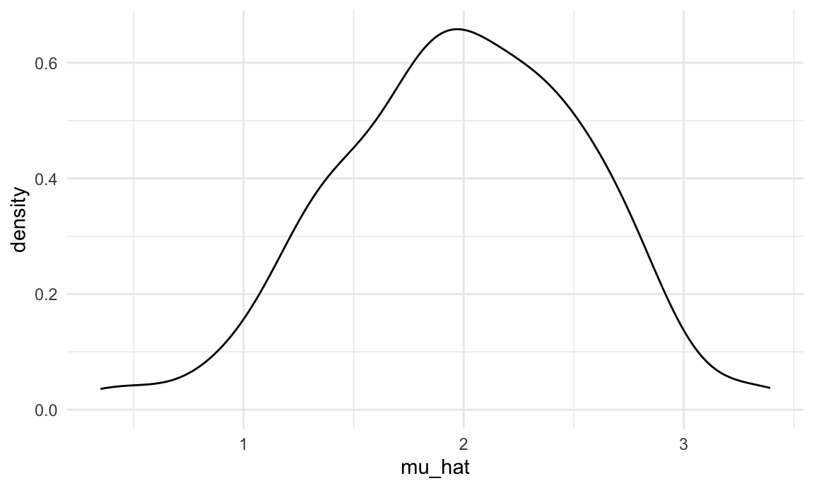

sim_results_df |> 
  pivot_longer(
    mu_hat:sigma_hat,
    names_to = "parameter", 
    values_to = "estimate") |> 
  group_by(parameter) |> 
  summarize(
    emp_mean = mean(estimate),
    emp_sd = sd(estimate)) |> 
  knitr::kable(digits = 3)

parameter	emp_mean	emp_sd
mu_hat	1.985	0.567
sigma_hat	2.979	0.384

This is great! We’ve seen how our estimates are distributed under our simulation scenario, and can compare empirical results to theoretical ones. In this way, we can build intuition for fundamental statistical procedures under repeated sampling in a way that’s not possible with single data sets.

In cases like this, where the inputs to the function don’t change, using an “anonymous” function can be a helpful shorthand. Here the syntax (i) defines a function with the input i, and that function just runs sim_mean_sd(30, 2, 3) without actually using i.

sim_results_df =   
  map(1:100, \(i) sim_mean_sd(30, 2, 3)) |> 
  bind_rows()

Simulation: Mean for several \(n\)s

Sample size makes a huge difference on the variance of estimates in SLR (and pretty much every statistical method). Let’s try to clarify that effect through simulating at a few sample sizes.

Building on the code above, I’ll set up a tibble with iterations and the sample sizes I want to investigate using expand_grid. From there, the steps are similar to they were before – we’ll apply the sim_mean_sd function to each iteration of each sample size and unnest the result.

sim_results_df = 
  expand_grid(
    sample_size = c(30, 60, 120, 240),
    iter = 1:1000
  ) |> 
  mutate(
    estimate_df = map(sample_size, sim_mean_sd)
  ) |> 
  unnest(estimate_df)

Let’s take a look at what we’ve accomplished in our simulations! First I’ll take a look at the distribution of mean estimates across sample sizes.

sim_results_df |> 
  mutate(
    sample_size = str_c("n = ", sample_size),
    sample_size = fct_inorder(sample_size)) |> 
  ggplot(aes(x = sample_size, y = mu_hat, fill = sample_size)) + 
  geom_violin()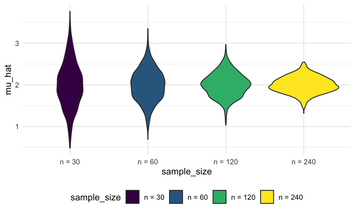

These estimates are centered around the truth (2) for each sample size, and the width of the distribution shrinks as sample size grows.

Lastly I’ll look at the empirical mean and variance of these estimates.

sim_results_df |> 
  pivot_longer(
    mu_hat:sigma_hat,
    names_to = "parameter", 
    values_to = "estimate") |> 
  group_by(parameter, sample_size) |> 
  summarize(
    emp_mean = mean(estimate),
    emp_var = var(estimate)) |> 
  knitr::kable(digits = 3)

## `summarise()` has grouped output by 'parameter'. You can override using the
## `.groups` argument.

parameter	sample_size	emp_mean	emp_var
mu_hat	30	2.001	0.289
mu_hat	60	1.992	0.147
mu_hat	120	2.005	0.079
mu_hat	240	1.999	0.038
sigma_hat	30	2.974	0.154
sigma_hat	60	2.999	0.068
sigma_hat	120	2.996	0.039
sigma_hat	240	2.994	0.018

These values are consistent with the formula presented for the distribution of the sample mean. This kind of check is a useful way to support derivations (although they don’t serve as a formal proof in any way).

Simulation: SLR for one \(n\)

The distribution of the sample mean is critical in statistics, but behaves in often familiar ways. Next we’ll use simulations to explore another very important setting that is sometimes surprising. In particular, we’ll use a function to we generate data from \[ y_i = \beta_0 + \beta_1 x_i + \epsilon_i \]

for subjects \(1 \leq i \leq n\) with \(\epsilon_i \sim N[0,1]\) and return estimates

\(\hat{\beta}_0, \hat{\beta}_1\).

One implementation of this goal is shown below. This takes the sample size and true regression coefficients as inputs; simulates both x and y; fits the regression; and returns the estimated coefficients.

sim_regression = function(n, beta0 = 2, beta1 = 3) {
  
  sim_data = 
    tibble(
      x = rnorm(n, mean = 1, sd = 1),
      y = beta0 + beta1 * x + rnorm(n, 0, 1)
    )
  
  ls_fit = lm(y ~ x, data = sim_data)
  
  tibble(
    beta0_hat = coef(ls_fit)[1],
    beta1_hat = coef(ls_fit)[2]
  )
}

As for the sample mean, the repeated sampling framework can be used to establish properties of estimates \(\hat{\beta}_0, \hat{\beta}_1\). If you could draw repeatedly from the population, your estimates will have a known mean and covariance:

\[ \hat{\beta}_0 \sim \left[\beta_0, \sigma^2 \left(\frac{1}{n} + \frac{\bar{x}}{\sum (x_i - \bar{x})^2}\right) \right] \mbox{ and } \hat{\beta}_1 \sim \left[\beta_1,\frac{\sigma^2}{\sum (x_i - \bar{x})^2} \right] \]

(Because our simulation design generates errors from a Normal distribution we also know that the estimates follow a Normal distribution, although that’s not guaranteed by least squares estimation.)

Again, though, “repeated sampling” remains conceptual for regression – but we can draw samples easily in simulations. We’ll use map to run sim_regression() 500 times and show the effect of randomness in \(\epsilon\) on estimates \(\hat{\beta}_0, \hat{\beta}_1\).

sim_results_df = 
  expand_grid(
    sample_size = 30,
    iter = 1:500
  ) |> 
  mutate(
    estimate_df = map(sample_size, sim_regression)
  ) |> 
  unnest(estimate_df)

Next we’ll plot the estimated coefficients against each other (\(\hat{\beta}_0\) on the x axis and \(\hat{\beta}_1\) on the y axis). Both estimators are “unbiased”, meaning that on average you get the right answer. But what’s striking about this plot is that the estimated coefficients are inversely correlated – a lower estimate of the intercept tends to imply a higher estimate of the slope.

sim_results_df |> 
  ggplot(aes(x = beta0_hat, y = beta1_hat)) + 
  geom_point()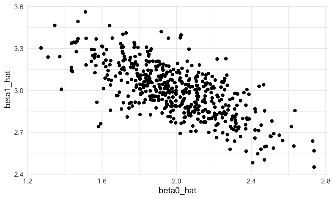

Varying two simulation parameters

In our last example, we’ll consider varying two parameters – the sample size and the true standard deviation in our simulation looking at the mean and SD. We can use expand_grid() again to consider all possible combinations of sample size and true SD, while also defining a variable to look at 1000 iterations of each combination.

The key step in this code chunk is the use of map2, which allows mapping over two inputs to a function. We can also use an “anonymous” function which passes inputs n and sd to specific arguments in the sim_mean_sd() function.

sim_results_df = 
  expand_grid(
    sample_size = c(30, 60, 120, 240),
    true_sd = c(6, 3),
    iter = 1:1000
  ) |> 
  mutate(
    estimate_df = 
      map2(sample_size, true_sd, \(n, sd) sim_mean_sd(n = n, sigma = sd))
  ) |> 
  unnest(estimate_df)

As before, once we have the results of this simulation, we can use graphical summaries to understand how the sample size and true SD relate to the distribution of the sample mean. For both true SDs, increasing the sample size results in a narrower distribution, and the distribution of the sample mean is wider when the true SD is larger.

sim_results_df |> 
  mutate(
    true_sd = str_c("True SD: ", true_sd),
    true_sd = fct_inorder(true_sd),
    sample_size = str_c("n = ", sample_size),
    sample_size = fct_inorder(sample_size)) |> 
  ggplot(aes(x = sample_size, y = mu_hat, fill = sample_size)) + 
  geom_violin() + 
  facet_grid(. ~ true_sd)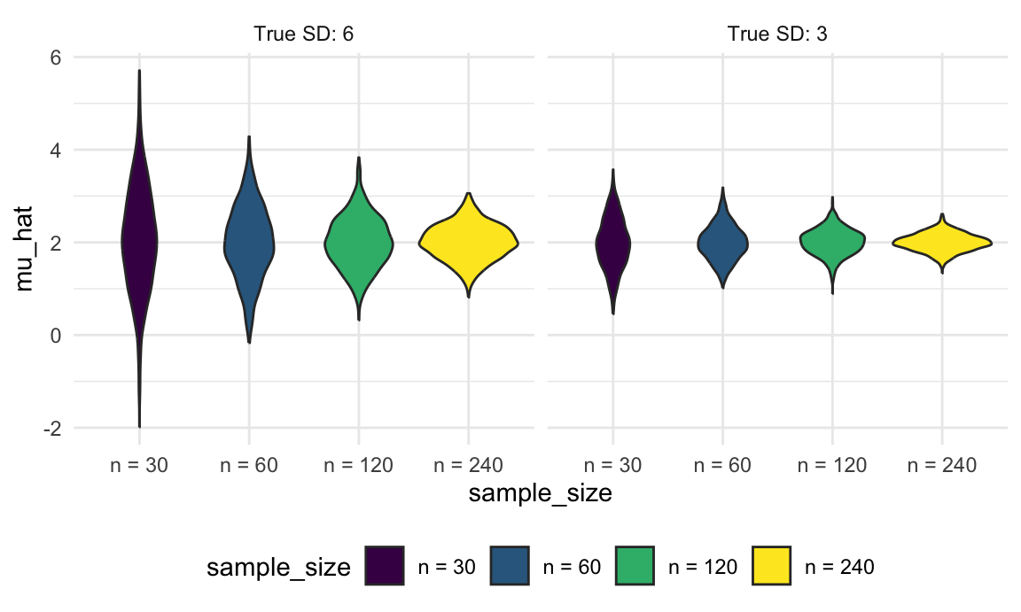

Other materials

• Problem of small power leading to over estimation has been discussed here among other places

The code that I produced working examples in lecture is here.

Copyright © 2019 Jeff Goldsmith