Tidy text
This is a bit of a diversion for a public-health-focused course in data science, but it’s fun, related to web data, strings, and factors, and emphasizes tools in data wrangling. It’s most closely related to content in the Data Wrangling II topic.
Overview
Learning Objectives
Use tidytext to organize text data, and to conduct
frequency and sentiment analyses.
Video Lecture
Example
I’ll write code for today’s content in a new R Markdown document
called tidy_text.Rmd, and put it in the extra topics
directory / GitHub repo. I’m going to load the tidyverse as
usual, as well as tidytext and rvest.
library(tidyverse)
library(tidytext)

library(rvest)
Data
We’re sticking with “Napoleon Dynamite reviews”! I’m showing code similar to that in iteration and listcols to scrape the 1000 most recent reviews on Amazon. Believe it or not, this code used to work – but then Amazon got real tired of everyone scraping their data all the time and set up stricter protections and an API for approved (paying) users.
read_page_reviews <- function(url) {

  html = read_html(url)

  review_titles =
    html |>
    html_nodes(".a-text-bold span") |>
    html_text()

  review_stars =
    html |>
    html_nodes("#cm_cr-review_list .review-rating") |>
    html_text() |>
    str_extract("^\\d") |>
    as.numeric()

  review_text =
    html |>
    html_nodes(".review-text-content span") |>
    html_text() |>
    str_replace_all("\n", "") |>
    str_trim()

  tibble(
    title = review_titles,
    stars = review_stars,
    text = review_text
  )
}

url_base = "https://www.amazon.com/product-reviews/B00005JNBQ/ref=cm_cr_arp_d_viewopt_rvwer?ie=UTF8&reviewerType=avp_only_reviews&sortBy=recent&pageNumber="

dynamite_reviews =
  tibble(
    page = 1:100,
    urls = str_c(url_base, page)) |>
  mutate(reviews = map(urls, read_page_reviews)) |>
  unnest(reviews) |>
  mutate(review_num = row_number()) |>
  relocate(page, review_num)
The output of the code above was a successfully scraped dataset with one row for each review. For each review we get the title of that review, the number of stars it received, and text that describers the users feelings about the movie.
In place of actually scraping the data, we can import this spreadsheet using the code
below. It’s not perfectly current but can illustrate the main ideas in
tidytext.
dynamite_reviews =
  read_csv("data/dynamite_reviews.csv")
## Rows: 1000 Columns: 4
## ── Column specification ───────────────────────────────────────────────────────────────────────────────
## Delimiter: ","
## chr (2): title, text
## dbl (2): review_num, stars
##
## ℹ Use `spec()` to retrieve the full column specification for this data.
## ℹ Specify the column types or set `show_col_types = FALSE` to quiet this message.Words and wordcounts
To illustrate tidy text and text analysis, we’ll focus on the reviews
directly, which are stored as strings in text. To begin our
analysis, we’ll un-nest the tokens (i.e. words) in each row; the result
is a tidy dataset in which each word is contained within a separate
row.
dynamite_words =
  dynamite_reviews |>
  unnest_tokens(word, text)
There are lots of words here that are uninformative. We’ll remove
“stop words” using anti_join; in other settings the words
you want to remove might be different.
data(stop_words)

dynamite_words =
  anti_join(dynamite_words, stop_words)
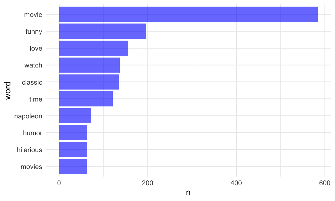
## Joining with `by = join_by(word)`Great! Let’s take a look at the most commonly used (informative) words in this dataset.
dynamite_words |>
  count(word, sort = TRUE) |>
  top_n(10) |>
  mutate(word = fct_reorder(word, n)) |>
  ggplot(aes(x = word, y = n)) +
  geom_bar(stat = "identity", fill = "blue", alpha = .6) +
  coord_flip()
## Selecting by n
Comparing words across groups
The next code chunk below produces a table of the most frequently used in one- and five-star reviews.
dynamite_words |>
  filter(stars %in% c(1, 5)) |>
  group_by(stars) |>
  count(word) |>
  top_n(5) |>
  knitr::kable()
## Selecting by n| stars | word | n |
|---|---|---|
| 1 | bad | 8 |
| 1 | dumb | 8 |
| 1 | dvd | 12 |
| 1 | movie | 51 |
| 1 | time | 10 |
| 1 | watch | 11 |
| 5 | classic | 114 |
| 5 | funny | 135 |
| 5 | love | 138 |
| 5 | movie | 437 |
| 5 | watch | 100 |
The table above gives the top 5 most frequently used words in 1-star and 5-star reviews. Movie is the most used word for both 1 and 5-star reviews, though other words, like dumb differentiate 1-star reviews from 5-star reviews, which have words like love.
Word frequency might be misleading because there are 762 5-star reviews and only 64 1-star reviews.
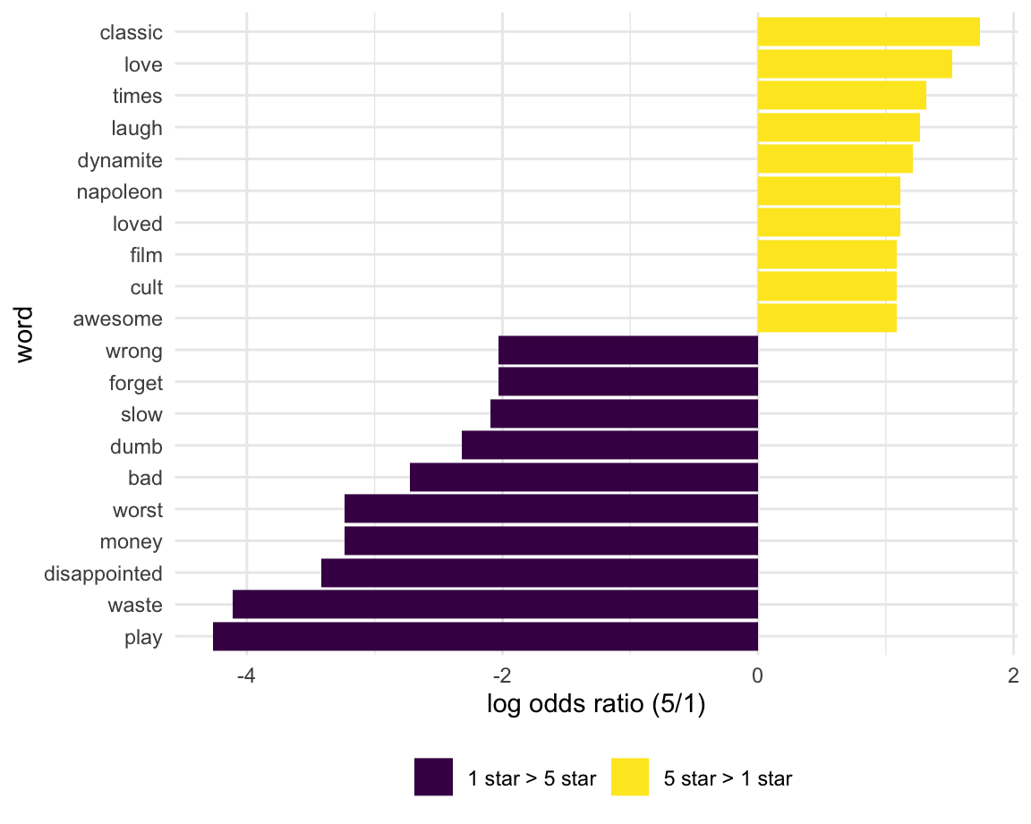
Let’s compare which words are more likely to come from a 1 versus 5 star ratings. We limit to words that appear at least 5 times and compute the approximate log odds ratio for each word.
word_ratios =
  dynamite_words |>
  filter(stars %in% c(1, 5)) |>
  count(word, stars) |>
  group_by(word) |>
  filter(sum(n) >= 5) |>
  ungroup() |>
  pivot_wider(
    names_from = stars,
    values_from = n,
    names_prefix = "stars_",
    values_fill = 0) |>
  mutate(
    stars_1_odds = (stars_1 + 1) / (sum(stars_1) + 1),
    stars_5_odds = (stars_5 + 1) / (sum(stars_5) + 1),
    log_OR = log(stars_5_odds / stars_1_odds)
  ) |>
  arrange(desc(log_OR))
Next, let’s plot the top 10 most distinctive words (that is, words that appear much more frequently in one group than the other) below.
word_ratios |>
  mutate(pos_log_OR = ifelse(log_OR > 0, "5 star > 1 star", "1 star > 5 star")) |>
  group_by(pos_log_OR) |>
  top_n(10, abs(log_OR)) |>
  ungroup() |>
  mutate(word = fct_reorder(word, log_OR)) |>
  ggplot(aes(word, log_OR, fill = pos_log_OR)) +
  geom_col() +
  coord_flip() +
  ylab("log odds ratio (5/1)") +
  scale_fill_discrete(name = "")
Words like “classic”, “awesome”, and “love” have high relative frequency in the 5-star reviews and “boring”, “dumb”, and “bad” have high relative frequency in the 1-star reviews. This seems to be a polarizing film.
Sentiment analysis
Finally, let’s score the sentiment in each word. We’ll use the “bing” (like Bing Liu, not like bing.com) sentiment lexicon, which simply categorizes each word as having a positive or negative sentiment.
bing_sentiments = get_sentiments("bing")Note this is might not always be appropriate – this scores
cold as negative which might not be accurate
for e.g. food inspections – but we’ll use it anyway.
We need to combine this lexicon with our tidy dataset containing words from each inspection. Note that only words that are in the sentiment lexicon will be retained, as the rest of the words are not considered meaningful. We’ll also count the number of positive and negative words in each review, and create a score that is the difference between the number of positive words and negative words.
dynamite_sentiments =
  dynamite_words |>
  inner_join(x = _, bing_sentiments) |>
  count(review_num, sentiment) |>
  pivot_wider(
    names_from = sentiment,
    values_from = n,
    values_fill = 0) |>
  mutate(review_sentiment = positive - negative) |>
  select(review_num, review_sentiment)
## Joining with `by = join_by(word)`We now have sentiment scores for each inspection. We’ll combine these with our original dataset, which had inspections in each row rather than words in each row – the data tidied for text analysis aren’t really suitable for our current needs.
dynamite_sentiments =
  right_join(
    dynamite_reviews, dynamite_sentiments,
    by = "review_num")
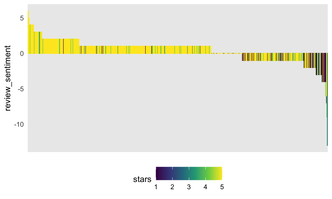
Finally, let’s make a plot showing inspection sentiments and stars.
dynamite_sentiments |>
  mutate(
    review_num = factor(review_num),
    review_num = fct_reorder(review_num, review_sentiment, .desc = TRUE)) |>
  ggplot(aes(x = review_num, y = review_sentiment, fill = stars, color = stars)) +
  geom_bar(stat = "identity") +
  theme(
    axis.title.x=element_blank(),
    axis.text.x=element_blank(),
    axis.ticks.x=element_blank())
Sentiment seems to be at least somewhat associated with star rating in that more positive sentiments are more yellow-green (4-5 stars) and more negative sentiments are more blue-purple.
Here is the text from the most positive review:
dynamite_sentiments |>
  filter(review_sentiment == max(review_sentiment)) |>
  pull(text)
## [1] "Love, love and love! My children ages 13, 10 and 8 enjoy family movie nights and my husband and I were looking for something that we all could enjoy. This movie was perfect! So much fun and beyond quotable comments. A fun family film!"
And here is the text from the most negative (1-star) review:
dynamite_sentiments |>
  filter(review_sentiment == min(review_sentiment), stars == 1) |>
  pull(text)
## [1] "Let me start by openly admitting that I am an 80's throwback and proud of it. I understand that my era did not produce horribly intelligent, deeply touching movies. That being said, this movie puts the Du-h! in Dumb!! My teenage daughter had seen it a sleepover, so we rented it so she could show me how silly it is for our girly night. She actually got tickled at a few spots on her second run through it. I sat open mouthed, amazed at the sheer senselessness of the whole thing...waiting desperately for a plot or growth of a character. None came. Since we had it rented for the weekend, she showed it to her older brother the next night. She giggled again, and he snickered with a confused look on his face once in a while. Then we couldn't let my Hubby miss out on the sheer stupidity of it all, so we watched it with him on Sunday afternoon. Our daughter and son both snickered here and there, mostly at the looks on their parents' faces. My husband was, as was I, gobsmackered. We kept looking at each other as if to assure each other that it was indeed that painfully dumb. The only real emotion I felt was a horribly heartbroken, sick to my stomach feeling for Napoleon and his friends for being so awkward and socially inept...I remember kids who struggled in school that way, and I always almost cried every time I saw them in a tough situation. If anything it brought back bad memories of school....who needs that? Anyway, all this to say it is a story about an awkward boy who uses bluster and dumb responses to deal with not fitting in. It follows (if you can exaggerate and say there is a plot) him as he finds friends (just as goofy as he) and finds romance...sort of."
Other materials
- The framework we used is explained in detail in the Tidy Text book
- One of the book’s authors, Julia Silge, has a nice video talking about the work
- The other of the book’s authors, Dave Robinson, used the approach to examine Donald Trump’s tweets in this this blog post
The code that I produced working examples in lecture is here.